Thursday 31 July 2014

Create a Motion Chart gadget using Google Sheets

***Update September 2017 - Google has now discontinued the motion chart, so the below solution will no longer work***


In Google Sheets, you have the option to simply create a chart and display this on your Google Site.  However, if you code this in a gadget, you have lots more potential to customise things. In this example I am using Google Sheet data for a motion chart, and customising the initial state that will display on my site.  A quick demo is below


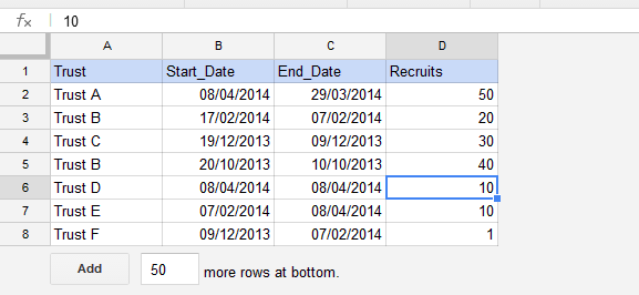
I found that motion charts do not load when the data range includes blank rows. For the data I am using which gets updated automatically each week using the method I blogged about here, the data range will grow over time, which causes a problem.   The solution to this is to use the QUERY function in Google sheets to bring in only the data in an IMPORTRANGE that contains valid data. This means you can specify a large range for the importrange to cover, but wont bring in any blank rows.

In the sheet that I want the motion chart to read from, I therefore applied the following formula,

=query(importrange("https://docs.google.com/a/nihr.ac.uk/spreadsheets/d/abcdefghijklmnopqrs1234567891011", "motion!Q2:S580"),"Select Col1, Col2, Col3 where Col3 > 0")

This extracts the data from my other Google sheet for the data I want to chart, only where the third column in the range (the values) are greater than zero.

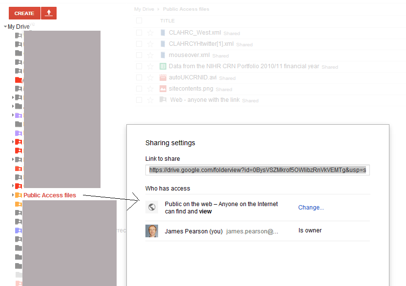
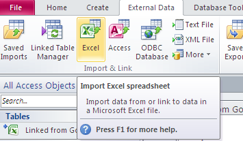
In my Google Sheet, I then went to File -> publish to the web, to make this data available for the gadget to read.

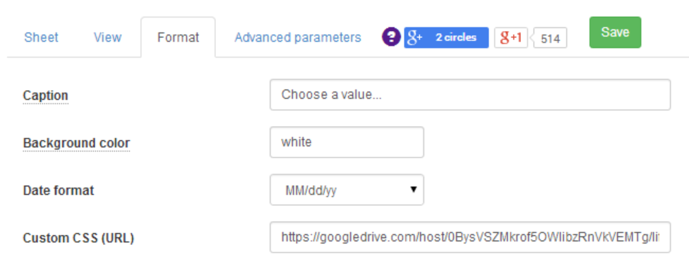
In the final chart I wanted to set the initial chart state as columns, with our network highlighted, and with unique colours for each network.  Once I applied these settings on the chart, by going to the advanced settings as per the below screenshot, it was possible to get the code for that state to then use in the gadget code so that when the chart loads, it will display exactly in this format.


Here's the completed gadget, with the live chart here:

<?xml version="1.0" encoding="UTF-8" ?>
<Module>
  <ModulePrefs title="Recruitment by LRN FY2014/5" width="600" height="500" scrolling="false">
    <Require feature="ads"/>
    <Require feature="flash"/>
  </ModulePrefs>
  <UserPref name="clickurl" datatype="hidden" default_value="DEBUG"/>
  <UserPref name="aiturl" datatype="hidden" default_value="DEBUG"/>
  <Content type="html"><![CDATA[
<head>
<script type="text/javascript" src="https://www.google.com/jsapi"></script>
<script type="text/javascript">
  google.load('visualization', '1', {'packages':['motionchart']});
google.setOnLoadCallback(drawChart);
function drawChart() {
  var query = new google.visualization.Query(
      'http://spreadsheets.google.com/tq?key=*****insert your key here******&pub=1');

  query.send(handleQueryResponse);
}

function handleQueryResponse(response) {
  if (response.isError()) {
    alert('Error in query: ' + response.getMessage() + ' ' + response.getDetailedMessage());
    return;
  }

  var data = response.getDataTable();
     var chart = new google.visualization.MotionChart(document.getElementById('motionchart'));
     
var options = {};
options['state'] =
'{"yZoomedDataMax":20000,"yLambda":1,"iconType":"VBAR","xAxisOption":"2","yZoomedDataMin":0,"dimensions":{"iconDimensions":["dim0"]},"iconKeySettings":[{"key":{"dim0":"NIHR CRN: Kent, Surrey and Sussex"}}],"nonSelectedAlpha":0.4,"orderedByX":true,"playDuration":15000,"showTrails":false,"orderedByY":false,"yZoomedIn":false,"xZoomedDataMin":0,"colorOption":"_UNIQUE_COLOR","time":"2014-04-01","xZoomedIn":false,"yAxisOption":"2","sizeOption":"_UNISIZE","xZoomedDataMax":15,"xLambda":1,"uniColorForNonSelected":false,"duration":{"timeUnit":"D","multiplier":1}};';

options['width'] = 600;
options['height'] = 500;
chart.draw(data, options);     
     
}
</script>


</head>

<body>
<span id='motionchart'></span>
</body>
       
  ]]></Content>
</Module>

(For details on how to upload a gadget and get the url to use on a Google site, see my blogpost here)

Thursday 24 July 2014

Tricks with Awesome Tables, Progress Bars, custom css and filtering Numbers

I am a huge fan of Romain Vialard's work especially his "Awesome Table Gadget" and use these extensively in my site for reporting.  This blog post shows some enhancements I have made to the out of the box gadget - my aim was to add coloured progress bars to demonstrate achievement to KPIs, to change the look and feel with some custom css, and to enable the table to be filtered by searching in a number field.

A demo of the completed table is here, which contains some dummy data.

Progress Bars

As the Awesome Tables can take HTML code and render this in the table, I wanted to produce a sample output such as this


The HTML code for this bar would be
"<div class=""PercentageBar_amber"">
<div class=""percent"" style=""width: 73&#37;;""><div class=""number"">73%</div></div>"

(The #37; is an encoded character for a % symbol which will render correctly in the table. The bar will have the class PercentageBar_amber - which allows for some custom css (which will be entered later) to target this div and change the background colour.)

To build this string up in the source sheet, I just used a formula to join together the sheet data and some HTML strings.

Custom CSS

For some tables, I wanted to make tweaks such as make the font size smaller, to enable more data to fit in to the view - for this example, I wanted to make two changes, firstly to create and colour the progress bars according to their rating, and secondly to change the colour of the header to look a bit better with the red template on my site.

To do this, I took first some sample css from Romain such as this one and then added some custom css at the end.  

/* Colour the header in red at the top and bottom */

.google-visualization-table-tr-head .gradient, .google-visualization-table-tr-head-nonstrict .gradient, .google-visualization-table-div-page .gradient {
    background: linear-gradient(to bottom, rgba(255, 78, 77, 0.95) 2%, rgba(255, 78, 77, 0.01) 7%, rgba(255, 78, 77, 0.04) 95%, rgba(255, 78, 77, 0.88) 6%) repeat scroll 0 0 rgba(42, 93, 41, 0) !important;
}


/* Progress Bars */

			.PercentageBar_red {position: relative; font-size: small; width: 100px; height: 14px; margin: 1px;}
			.PercentageBar_red DIV {height: 9px; line-height: 6px;}
			.PercentageBar_red .percent {position: relative; background-color: #ee7980; left: 0px top: 0px; z-index: 0;border: 1px solid;}
			.PercentageBar_red .caption {position: relative; text-align: center; color: #000; z-index: 1;}
			
			
			.PercentageBar_green {position: relative; font-size: small; width: 100px; height: 14px; margin: 1px;}
			.PercentageBar_green DIV {height: 9px; line-height: 6px;}
			.PercentageBar_green .percent {position: relative; background-color: #55e84c; left: 0px top: 0px; z-index: 0;border: 1px solid;}
			.PercentageBar_green .caption {position: relative; text-align: center; color: #000; z-index: 1;}


			.PercentageBar_amber {position: relative; font-size: small; width: 100px; height: 14px; margin: 1px;}
			.PercentageBar_amber DIV {height: 9px; line-height: 6px;}
			.PercentageBar_amber .percent {position: relative; background-color: #fcc564; left: 0px top: 0px; z-index: 0;border: 1px solid;}
			.PercentageBar_amber .caption {position: relative; text-align: center; color: #000; z-index: 1;}
			
						.PercentageBar_black {position: relative; font-size: small; width: 100px; height: 14px; margin: 1px;}
			.PercentageBar_black DIV {height: 9px; line-height: 6px;}
			.PercentageBar_black .percent {position: relative; background-color: #000000; left: 0px top: 0px; z-index: 0;border: 1px solid;}
			.PercentageBar_black .caption {position: relative; text-align: center; color: #000; z-index: 1;}
			
						.PercentageBar_blue {position: relative; font-size: small; width: 100px; height: 14px; margin: 1px;}
			.PercentageBar_blue DIV {height: 9px; line-height: 6px;}
			.PercentageBar_blue .percent {position: relative; background-color: #91C0EF; left: 0px top: 0px; z-index: 0;border: 1px solid;}
			.PercentageBar_blue .caption {position: relative; text-align: center; color: #000; z-index: 1;}
			
	.number {
    font-size: small;
    position: absolute;
    text-align: right;
}

In the Awesome table setup screen, you can add this custom css in. I just saved the css file to my Google Drive in a public folder and found the published URL. Please see my blog post here if you need more details on how to do this (it works the same for css as gadgets)

Searching a Number field

One small annoyance with Awesome tables, is that if you have a numerical field, you can only have a filter that is a range filter (like a slider) or not filter it at all.  This may be appropriate sometimes, but for situations where you need to look for something like a Study ID or a part number for example, it really does not work well.  The workaround I have found works is as follows

In my Google Sheet, I have new column with a  formula which concatenates some text e.g. "StudyID" and the actual number. So instead of 123 this becomes StudyID123

Filter terms in an Awesome table can be combined, for example,  "CategoryFilter - Hidden" will do a dropdown filter for that column, but wont show that column in the table.   The trick therefore is to have your original number column as "NoFilter"  (so it displays in the table)  and for the newly created concatenated column, the filter "StringFilter - Hidden".  

With this in place, you can then search for rows containing a specific number


Tuesday 27 May 2014

Updating Google Sheets and Awesome tables with Access queries

Each week I need to update charts and tables on a Google site using data that I have processed locally in MS Access.
         In the absence of being able currently to connect my local MS Access database direct to Google via JDBC or similar, I have found a method of updating Google Sheets and related Awesome tables with Access data, which uses a combination of Drive, Google Apps Script and a Google Sheet.

The idea of this is that the new exports from Access are saved to a specific drive folder each week then a script is run from a master Google sheet which looks for these specific file names and finds the new keys, With these keys identified, the sheet then can use a standard IMPORTRANGE function to bring in the new applicable data.  This then automatically updates Awesome tables and charts on a Google site linked to that master Google sheet.


To start, I export all the relevant Access queries to my local drive, and then uploaded and converted these to Google sheets format to a specific Drive folder which is accessible by anyone with the link. (I also delete the old files that these are intended to replace)

On my master Google sheet, I have a sheet called "FindKeys" - The script looks for a specific drive folder (e.g. abcdefghijk12345678 in the below) and then lists the file names and the spreadsheet keys for each item in the sheet

function search()  {


    var folder =  DriveApp.getFolderById("abcdefghijk12345678");
    
  var files = folder.getFiles();
  
   
     var sheetName = 'FindKeys';
     
var SheetIds = 2;

var sheet = SpreadsheetApp.getActiveSpreadsheet().getSheetByName(sheetName);

  sheet.clear();

  sheet.appendRow(["FileName","SpreadsheetKey"]);

 while (files.hasNext()) {

   var file = files.next();
   Logger.log(file);
 var data;
    data = [
     file.getName(),
  file.getId(),
    ];

    sheet.appendRow(data);

  }
};


Since I now have the spreadsheet keys, I can use a simple Vlookup formula on another sheet, to return the keys for only the specific queries that I am interested in.


Since the cell reference of each key that is found will not change, these can then be used in another sheet to bring in the data using IMPORTRANGE.   In the example below, I have this formula on row 3, which allows me to use rows 1 and 2 in the right format for this data to be easily used in an Awesome Table


My master sheet contains a number of these IMPORTRANGE queries  - this allows me to update all the tables at once from this master sheet.  I just need to open the master sheet, run the script to identify the current keys, and after 30 seconds or so, all the reports will update to the latest data based from the current Access queries and show in an Awesome table on my Google site.


This process could be made even more automated by running a script with a timer, to rebuild the Importrange formulae on a regular basis - for my purposes as this is a weekly job, I am happy to keep the manual step of opening up the master sheet each week to do the updates

Hope this is of use - any questions or suggestions welcomed

Friday 9 May 2014

How to host a gadget on Google Drive

To add a gadget such as a twitter widget into a Google Site, it is necessary to host the gadget file that you create somewhere.  Although in the past I used to host these gadgets on external websites, or via Dropbox, it is possible to use your Google Drive to host the gadget instead.

To do this, I created a folder in Google Drive, and set the sharing permissions for that folder to public on the web


I then uploaded a gadget containing the Twitter Widget code to that folder.

To get the URL that is required on a site when using the 'Add Gadget by URL' option,  In Drive, I clicked on the "Details and Activity" Button   and selected the Details pane


In this pane, there is a link to the hosting path for the files in this folder.  Clicking this link should take you to a folder view, where you can click on any of the files to get the URL


Clicking on the gadget gives a display of the file and the URL you need to copy and use


Using this link on a Google site, 'Add Gadget by URL' will then bring this through.


Thursday 1 May 2014

Interactive reports using QUERY and IMPORTRANGE

Using the formula =IMPORTRANGE in a Google sheet allows you to easily bring through data from other sheets. For some more powerful functions you can combine QUERY and IMPORTRANGE as in the examples below, and make these interactive using dropdowns or values directly entered in a cell

On one sheet I have uploaded some historical data on NIHR Trust performance, published on the Guardian's Clinical Research Zone.  I will then use this spreadsheet as the source to bring in selected data on another target sheet.

In the first example, using data validation, I have put in a dropdown in cell B3 containing all the different trust types.  Using the following formula, I can then return the list of trusts that match exactly the value selected in that cell:

=(QUERY(IMPORTRANGE("15Q9ppH0-Pcdwak0Eyns4NNtMMv0Ft0PeqGf2RDfWot4","A:k"),"SELECT Col1, Col2, Col4 WHERE Col3 =" & "'" & B3 & "'"))


In the next example, I have amended the dropdown to include some shorter keywords, that will match more items.  I have then adjusted the formula, so that it does not look for an 'equals' match, but instead a 'contains'

=(QUERY(IMPORTRANGE("15Q9ppH0-Pcdwak0Eyns4NNtMMv0Ft0PeqGf2RDfWot4","A:k"),"SELECT Col1, Col2, Col4 WHERE Col3 CONTAINS" & "'" & B3 & "'"))


In the next example, I wanted to show all the trusts that have above a certain number of recruiting studies. Instead of a dropdown, I just have a cell that users can type a number in.   The formula for this one is:

=(QUERY(IMPORTRANGE("15Q9ppH0-Pcdwak0Eyns4NNtMMv0Ft0PeqGf2RDfWot4","A:k"),"SELECT Col1, Col2, Col7 WHERE Col7 >"&B3))


In the final example, I wanted to use a SUM function, to calculate the total number of studies for each of the trust types, and apply a custom title/label "Total number of studies" to that column.  The formula for this is

=(QUERY(IMPORTRANGE("15Q9ppH0-Pcdwak0Eyns4NNtMMv0Ft0PeqGf2RDfWot4","A:k"),"SELECT Col3, sum(Col7) where Col3 contains"& "'" & B3 & "'" &"Group by Col3 label sum(Col7) 'Total number of studies' "))


NB - a quirk of the new Google sheets, is that you need to authorise a connection between the source and the target sheet when you do an IMPORTRANGE.   When you use a standard IMPORTRANGE, it gives an error and prompts you to do this as in the screenshot below:
Unless you have already made this connection, using IMPORTRANGE the QUERY(IMPORTRANGE(  function will not work.  To enable this to work for my demo sheet, all I needed to do was a simple IMPORTRANGE formula on another sheet such as:
=importrange("15Q9ppH0-Pcdwak0Eyns4NNtMMv0Ft0PeqGf2RDfWot4","B:B")
Once the connection has been authorised, the other formulae will work as expected.
  

A copy of the sheet with the formulae in can be downloaded here:


Friday 25 April 2014

Create and share customised templates linked to a master collection sheet

There are lots of times when it would be useful to create batches of sheets with customised information, share these with specified people automatically, and have any changes that those users make, automatically collected and visible from one master sheet.

I have created a variant of this script to collect a large volume of information from 200+ organisations, but am going to demo a simpler version here, which aims to create individual annual leave sheets for all staff, populating each one with data relevant to each person, sharing these with them individually, and allowing the main administrator to see at a glance what the remaining balances of holidays are for everyone as time goes on and the staff update their sheets.

To start, I created a simple sheet - shown here with some sample data:


The Spreadsheet IDs and Email Sent cells will get populated automatically once the script runs.
The Current Balances and Link to Spreadsheets are generated using formulae (importrange and a hyperlink concatenation respectively)

I also created a separate template sheet workbook (below), which the script will customise using the information on the master sheet above, make a copy, then share with the appropriate staff members.


For the Scripts, I created a couple of menu entries that will appear when the master sheet loads


function onOpen() {
var ss = SpreadsheetApp.getActiveSpreadsheet();
  var menuEntries = [{
    name: "Generate Annual Leave Sheets",
    functionName: "CreateAnnualLeaveSheets"
  }, 
    {
    name: "Send Emails",
    functionName: "sendEmails"
    }];
  ss.addMenu("Run Annual Leave Scripts", menuEntries);
}

Next I created the main script, which will create a customised copy of each template and share it with the user whose email address is in column B

var ss = SpreadsheetApp.getActiveSpreadsheet();
var sheetName = 'Master'; //I renamed Sheet1! to Master
var SheetIds = 3;  //this is the column to store the generated sheet IDs

function CreateAnnualLeaveSheets(){
  var sheet = SpreadsheetApp.getActiveSpreadsheet().getSheetByName(sheetName);
  //use the id of the template sheet
  var sstemplate = SpreadsheetApp.openById("**************************"); //replace with your template key
  var data = sheet.getDataRange().getValues();
  for(var i = 1; i < data.length; i++){
    if(data[i][0] != '' && (data[i][SheetIds-1] == '' || !data[i][SheetIds-1])) {
    
     var reportname = data[i][0];  // this is column A (A=0, B=1, C=2 etc.)
     var AdditionalEditor = data[i][1];  //column B  - the email that template will be shared with
     var Name = data[i][5];  // column F   - their name
      var Department = data[i][6];  //column G  - their department
     
      var Basic = data[i][7];  //column H   - number of days annual leave
      var cfwd = data[i][8];  //column I   - number of days carried forward
     
      
       sstemplate.getSheetByName("Sheet1").getRange('B2').setValue(Name);   // append name to the template
       sstemplate.getSheetByName("Sheet1").getRange('B3').setValue(Department); // append department 
        sstemplate.getSheetByName("Sheet1").getRange('B4').setValue(Basic);  // append no. days basic
         sstemplate.getSheetByName("Sheet1").getRange('B5').setValue(cfwd);  //append no days carried forward
      
      var newsheet = sstemplate.copy(reportname).getId();  //create a copy of the template and save it with the report name
           sheet.getRange(i+1, SheetIds).setValue(newsheet);  // write the newly created key to the master sheet
        var newsheeteditors = SpreadsheetApp.openById(newsheet);  // open each sheet
        newsheeteditors.addEditors([AdditionalEditor]);   // assign edit rights to the named person
    
    }
    
  } //loop
 
}


When this script is run, the spreadsheet keys all fill in automatically on the master sheet. This allows us also to reference each of the keys in a formula, to bring in selected data to the master.  In this case I just wanted to see the outstanding holiday balance for each staff member.  For this I just needed a formula such as:

=if(C2<>"",importrange("https://docs.google.com/a/****/spreadsheets/d/"&C2,"Sheet1!$G$2"),"")

This formula allows cell G2 from each of the staff sheets to be brought through to the master sheet.
Whereas old sheets limited you to 50 Importrange formulae, new sheets has no limit, but it does require you to authorise each data connection. You only have to do this once for each of the linked sheets, so you can have multiple importranges to the same child sheet, which will all work as soon as just one of them is authorised.


I just used conditional formatting for the cell to go red if there is an error (such as if the sheets are not yet connected) Once you have clicked on "Allow Access"  the data should come through from then on.


I also have an email script that is designed to contact each of the staff members, informing them that a sheet has been created in their 'Shared with me' folder, with a link direct to the sheet for convenience.

//allow specific text to be written to sheet to prevent duplicate emails being sent
var EMAIL_SENT = "EMAIL_SENT";

function sendEmails() {
  var sheet = SpreadsheetApp.getActiveSheet();
  var startRow = 2;  // First row of data to process
  var numRows = 21;   // Number of rows to process
  // Fetch the range 
  var dataRange = sheet.getRange(startRow, 1, numRows, 12)
  // Fetch values for each row in the Range.
  var data = dataRange.getValues();
  for (var i = 0; i < data.length; ++i) {
    var row = data[i];
    var emailAddress = row[1];  // seccond column  (Column B)
    var message = row[10];       // column K
    var emailSent = row[9];     // column J  
    if (emailSent != EMAIL_SENT) {  // Prevents sending duplicates
      var subject = row[0];     //  column (A)
      Logger.log(emailAddress);
      MailApp.sendEmail(emailAddress, subject, message);
      sheet.getRange(startRow + i, 10).setValue(EMAIL_SENT);
      // Make sure the cell is updated right away in case the script is interrupted
      SpreadsheetApp.flush();
    }
  }
}


function SheetFlush(worksheet) {
    worksheet = worksheet || SpreadsheetApp.getActive();
    var sheets = worksheet.getSheets();
    SpreadsheetApp.flush();
}


You can customise the body and title using text and formulae on the master sheet, on mine, the end result looks something like this.


Variations of this script can be used to send regular customised reports out to large numbers of users, or to send complex data collection sheets that may need to be worked on over longer periods of time.

Hope it is of use, any questions or feedback welcomed


Tuesday 8 April 2014

Linking Google Sheet data to MS Excel and MS Access

With SharePoint I used to link lists to both Excel and Access quite frequently.  Although Google Sheets does not have the two way interactivity that has been so useful, it is still possible to have data that is entered on a Google Sheet, to be automatically imported and refreshed to a local Excel workbook.  In addition, its possible to use Excel as a bridge to then get Access to use that data.

Link a Google Sheet to Excel

To bring in Google Sheet data to Excel, you need to do a web query in Excel


Enter the URL of your Google Sheet and tick the green box to the left to select the sheet data


This return you something like this in Excel

A B C D E F
1
Trust Start_Date End_Date Recruits п»ї п»ї
2
Trust A 08/04/2014 29/03/2014 50 п»ї п»ї
3
Trust B 17/02/2014 07/02/2014 20 п»ї п»ї
4
Trust C 19/12/2013 09/12/2013 30 п»ї п»ї
5
Trust B 20/10/2013 10/10/2013 40 п»ї п»ї
6
Trust D 08/04/2014 08/04/2014 10 п»ї п»ї
7
Trust E 07/02/2014 08/04/2014 10 п»ї п»ї
8
Trust F 09/12/2013 07/02/2014 1 п»ї п»ї
9
п»ї п»ї п»ї п»ї п»ї п»ї
10
п»ї п»ї п»ї п»ї п»ї п»ї
11
п»ї п»ї п»ї п»ї п»ї п»ї
12
п»ї п»ї п»ї п»ї п»ї п»ї
13
п»ї п»ї п»ї п»ї п»ї п»ї
14
п»ї п»ї п»ї п»ї п»ї п»ї
15
п»ї п»ї п»ї п»ї п»ї п»ї
16
п»ї п»ї п»ї п»ї п»ї п»ї

As you can see, for any blank cells, these produce "п»ї"  symbols.   You can either hide these with conditional formatting in Excel, or to be much cleaner, just delete empty rows and columns in Google Sheets. If you need to add new data in the Google sheet at any time, its easy just to create new rows as required.

After deleting the unused rows and columns in Google sheets, it now looks like this

In Google Sheets


In Excel


The data in Excel can be refreshed manually by right clicking on the data and clicking refresh, or if you want this to be automatic whenever the sheet is opened, you can right click in the data, and click "Data Range Properties"  clicking the box "refresh data when opening the file"


This should now give you a live link to the Google Sheet data.

Synchronising with MS Access

In Access, you can link an Excel workbook as an Access Table, allowing the data to be then used in queries.

To link in your Excel workbook which contains the linked data from Google Sheets, open Access, and Import and Link as per the below screenshot


Choose the following radio button option


When you have completed the import, you should now see your Google Sheet data, as a table.


As you can see from the above example, Access has recognised numerical and date fields, and my headers for these rows come across as errors.   If you have the same issue, this can easily be sorted in a simple query based from this data as in the below:

Design view:


Datasheet view:


To refresh data from Google sheets therefore, you would just need to open your Excel workbook, allow the refresh from Google to complete, and then open your Access Database, and pull in the new data automatically.  If you wanted, with a few lines of VB you could also get Access to open the Excel workbook when it opens and before it runs queries on the new data.

Please let me know your feedback on this, especially if you encounter any bugs!