Tuesday 27 May 2014

Updating Google Sheets and Awesome tables with Access queries

Each week I need to update charts and tables on a Google site using data that I have processed locally in MS Access.
         In the absence of being able currently to connect my local MS Access database direct to Google via JDBC or similar, I have found a method of updating Google Sheets and related Awesome tables with Access data, which uses a combination of Drive, Google Apps Script and a Google Sheet.

The idea of this is that the new exports from Access are saved to a specific drive folder each week then a script is run from a master Google sheet which looks for these specific file names and finds the new keys, With these keys identified, the sheet then can use a standard IMPORTRANGE function to bring in the new applicable data.  This then automatically updates Awesome tables and charts on a Google site linked to that master Google sheet.


To start, I export all the relevant Access queries to my local drive, and then uploaded and converted these to Google sheets format to a specific Drive folder which is accessible by anyone with the link. (I also delete the old files that these are intended to replace)

On my master Google sheet, I have a sheet called "FindKeys" - The script looks for a specific drive folder (e.g. abcdefghijk12345678 in the below) and then lists the file names and the spreadsheet keys for each item in the sheet

function search()  {


    var folder =  DriveApp.getFolderById("abcdefghijk12345678");
    
  var files = folder.getFiles();
  
   
     var sheetName = 'FindKeys';
     
var SheetIds = 2;

var sheet = SpreadsheetApp.getActiveSpreadsheet().getSheetByName(sheetName);

  sheet.clear();

  sheet.appendRow(["FileName","SpreadsheetKey"]);

 while (files.hasNext()) {

   var file = files.next();
   Logger.log(file);
 var data;
    data = [
     file.getName(),
  file.getId(),
    ];

    sheet.appendRow(data);

  }
};


Since I now have the spreadsheet keys, I can use a simple Vlookup formula on another sheet, to return the keys for only the specific queries that I am interested in.


Since the cell reference of each key that is found will not change, these can then be used in another sheet to bring in the data using IMPORTRANGE.   In the example below, I have this formula on row 3, which allows me to use rows 1 and 2 in the right format for this data to be easily used in an Awesome Table


My master sheet contains a number of these IMPORTRANGE queries  - this allows me to update all the tables at once from this master sheet.  I just need to open the master sheet, run the script to identify the current keys, and after 30 seconds or so, all the reports will update to the latest data based from the current Access queries and show in an Awesome table on my Google site.


This process could be made even more automated by running a script with a timer, to rebuild the Importrange formulae on a regular basis - for my purposes as this is a weekly job, I am happy to keep the manual step of opening up the master sheet each week to do the updates

Hope this is of use - any questions or suggestions welcomed

Friday 9 May 2014

How to host a gadget on Google Drive

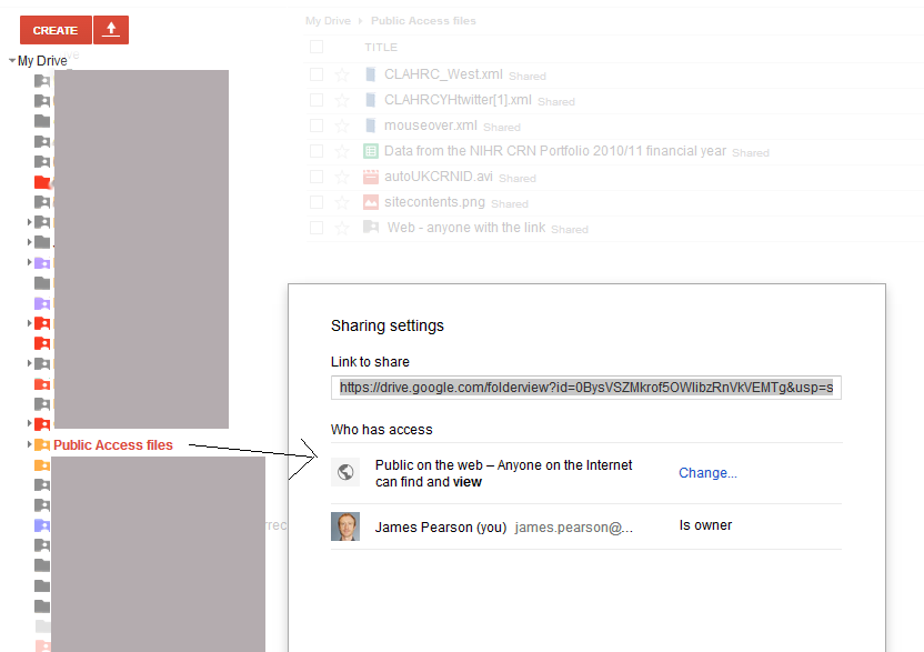
To add a gadget such as a twitter widget into a Google Site, it is necessary to host the gadget file that you create somewhere.  Although in the past I used to host these gadgets on external websites, or via Dropbox, it is possible to use your Google Drive to host the gadget instead.

To do this, I created a folder in Google Drive, and set the sharing permissions for that folder to public on the web


I then uploaded a gadget containing the Twitter Widget code to that folder.

To get the URL that is required on a site when using the 'Add Gadget by URL' option,  In Drive, I clicked on the "Details and Activity" Button   and selected the Details pane


In this pane, there is a link to the hosting path for the files in this folder.  Clicking this link should take you to a folder view, where you can click on any of the files to get the URL


Clicking on the gadget gives a display of the file and the URL you need to copy and use


Using this link on a Google site, 'Add Gadget by URL' will then bring this through.


Thursday 1 May 2014

Interactive reports using QUERY and IMPORTRANGE

Using the formula =IMPORTRANGE in a Google sheet allows you to easily bring through data from other sheets. For some more powerful functions you can combine QUERY and IMPORTRANGE as in the examples below, and make these interactive using dropdowns or values directly entered in a cell

On one sheet I have uploaded some historical data on NIHR Trust performance, published on the Guardian's Clinical Research Zone.  I will then use this spreadsheet as the source to bring in selected data on another target sheet.

In the first example, using data validation, I have put in a dropdown in cell B3 containing all the different trust types.  Using the following formula, I can then return the list of trusts that match exactly the value selected in that cell:

=(QUERY(IMPORTRANGE("15Q9ppH0-Pcdwak0Eyns4NNtMMv0Ft0PeqGf2RDfWot4","A:k"),"SELECT Col1, Col2, Col4 WHERE Col3 =" & "'" & B3 & "'"))


In the next example, I have amended the dropdown to include some shorter keywords, that will match more items.  I have then adjusted the formula, so that it does not look for an 'equals' match, but instead a 'contains'

=(QUERY(IMPORTRANGE("15Q9ppH0-Pcdwak0Eyns4NNtMMv0Ft0PeqGf2RDfWot4","A:k"),"SELECT Col1, Col2, Col4 WHERE Col3 CONTAINS" & "'" & B3 & "'"))


In the next example, I wanted to show all the trusts that have above a certain number of recruiting studies. Instead of a dropdown, I just have a cell that users can type a number in.   The formula for this one is:

=(QUERY(IMPORTRANGE("15Q9ppH0-Pcdwak0Eyns4NNtMMv0Ft0PeqGf2RDfWot4","A:k"),"SELECT Col1, Col2, Col7 WHERE Col7 >"&B3))


In the final example, I wanted to use a SUM function, to calculate the total number of studies for each of the trust types, and apply a custom title/label "Total number of studies" to that column.  The formula for this is

=(QUERY(IMPORTRANGE("15Q9ppH0-Pcdwak0Eyns4NNtMMv0Ft0PeqGf2RDfWot4","A:k"),"SELECT Col3, sum(Col7) where Col3 contains"& "'" & B3 & "'" &"Group by Col3 label sum(Col7) 'Total number of studies' "))


NB - a quirk of the new Google sheets, is that you need to authorise a connection between the source and the target sheet when you do an IMPORTRANGE.   When you use a standard IMPORTRANGE, it gives an error and prompts you to do this as in the screenshot below:
Unless you have already made this connection, using IMPORTRANGE the QUERY(IMPORTRANGE(  function will not work.  To enable this to work for my demo sheet, all I needed to do was a simple IMPORTRANGE formula on another sheet such as:
=importrange("15Q9ppH0-Pcdwak0Eyns4NNtMMv0Ft0PeqGf2RDfWot4","B:B")
Once the connection has been authorised, the other formulae will work as expected.
  

A copy of the sheet with the formulae in can be downloaded here: