The National Institute of Health Research (NIHR) publish an annual table of national research activity. In this demo, I am going to use this dataset in Google sheets, by extracting a subset of the information from the website with a formula, and then using a few different pivot formula to manipulate the data.
The table is published on the webpage here
Importhtml
To extract just the information for NHS organisations in Kent, Surrey and Sussex, in my Google sheet I have used the formula=query(importhtml("http://www.nihr.ac.uk/research-and-impact/nhs-research-performance/league-tables/league-table-data.htm", "table",1),"SELECT Col1, Col2, Col3,Col4,Col5,Col6,Col7,Col8 where Col3 ='Kent, Surrey and Sussex'")

Simple pivot
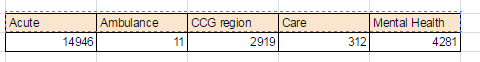
To pivot the results, you can use a pivot table in Google sheets, via the data menu, However you can also use a formula to generate a pivotHere's a simple example (where the raw data is on a sheet called "Raw Data 1" - showing the number of recruits by organisation type.
=query('Raw Data 1'!A:H, "select sum(H) pivot B")
Transpose a pivot
To change the orientation, so that it looks more like a normal pivot table, you can use 'transpose' in the formula=transpose(query('Raw Data 1'!A:H, "select sum(H) pivot B"))

Filter a pivot
You can also apply a filter parameter in your query, so for example the following shows the sum of recruitment for just Acute trusts=transpose(query('Raw Data 1'!A:H, "select sum(H) where B ='Acute' pivot A "))

Use multiple columns in a pivot
You can also bring other columns into a pivot, as long as these are included in the 'group by' or wrapped in an aggregate function. I have used a 'where' clause too to prevent blank rows being included in the pivot=query('Raw Data 1'!A:H, "select A,sum(H) where G >0 group by A pivot B")

Sorting a pivot
Sorting a pivot is more tricky, in the example below, I have used a query, to query the query ;-)=QUERY( TRANSPOSE((query('Raw Data 1'!A:H, "select sum(H) where B ='Acute' pivot A"))) , "Select Col1,Col2 Order by Col2 desc ")
